Using scispaCy for Named-Entity Extraction: A step-by-step tutorial for extracting data from biomedical literature
In 2019, the Allen Institute for Artificial Intelligence (AI2) developed scispaCy, a full, open-source spaCy pipeline for Python designed for analyzing biomedical and scientific text using natural language processing (NLP). scispaCy is a powerful tool, especially for named entity recognition (NER), or identifying keywords (entities) and classifying them into categories. I will be taking you through a basic introduction to using scispaCy for NER, and you will soon be on your way to becoming a master of NLP.
Agenda
- Set up Environment
- Install pandas
- Choose a model
- Import Packages
- Import Data
- Select Data
- Implementing Named-Entity Recognition
- Larger Data
Setting Up an Environment
The first step is to choose an environment to work in. I used Google Colab, but Jupyter Notebook or simply working from the terminal are fine, too. If you do work from the terminal, just make sure to create a virtual environment to work in. If you are working in Google Colab, there is no need to do this. Easy-to-follow instructions on creating a virtual environment can be found here.
Because I used Google Colab, the syntax used may be slightly different than that used for other environments.
The Google Colab for this project can be found here.
Installing pandas
Pandas is a Python library used for data manipulation. This will help with importing and representing the data we will analyze (talked about in the next section). If you’re working from Google Colab, pandas comes pre-installed, so you can ignore this step. Otherwise, install pandas using either Conda or PyPI (whichever you prefer). You can view all the steps for the installation process here.
Installing scispaCy
Installing scispaCy is pretty straight-forward. It is installed just like any other Python package.
!pip install -U spacy
!pip install scispacy
Picking a Pre-trained scispaCy Model
After installing scispaCy, you next need to install one of their premade models. scispaCy models come in two flavors: Core and NER. The Core models come in three sizes (small, medium, large) based on the amount of vocabulary stored, and they identify entities but do not classify them. The NER models, on the other hand, identify and classify entities. There are 4 different NER models built on different entity categories. You may need to experiment with the different models to find which one works best for your needs. The full list of models and specifications can be found here. Once you pick a model, install it using the model URL.
!pip install https://s3-us-west-2.amazonaws.com/ai2-s2-scispacy/releases/v0.2.4/en_core_sci_sm-0.2.4.tar.gz
Example of installing the “en_core_sci_sm” model
Import your packages
Once you have installed all of your packages and a virtual environment is created, simply import the packages you just downloaded.
import scispacy
import spacy
import en_core_sci_sm
from spacy import displacy
import pandas as pd
You may notice we also import an additional package “displacy”. Displacy isn’t required in order to perform any of the NER actions, but it is a visualizer that helps us see what’s going on.
Importing Data
For this example, we used the metadata from CORD-19, an open database of research papers about Covid-19. The metadata, as well as the full collection of articles, can be found here.
To import the data, we use the pandas read_csv() function.
df = pd.read_csv(“content/sample_data/metadata.csv”)
The function reads in the file path and stores the data as a DataFrame, the main Pandas data structure. For more information on how pandas stores and manipulates data, you can view the documentation here.
If you are using Colab, you can drag the file into the “Files” section, then right-click and choose “Copy path” to easily access the path to the file you want.
Selecting the Relevant Data
The metadata provides lots of useful information about the over 60,00 papers in CORD-19, including authors, reference numbers, etc. However, for our purposes, the data we care about is the abstracts. The full abstract of each paper is listed under the column named “abstract”. So, our next step is to choose this text. We will do this using the DataFrame loc function. This function takes in the location of a cell in the DataFrame and returns the data present in that cell. To access a specific abstract, just type the specific row you want and the header of the column, and store as a string variable.
text = meta_df.loc[0, “abstract”]
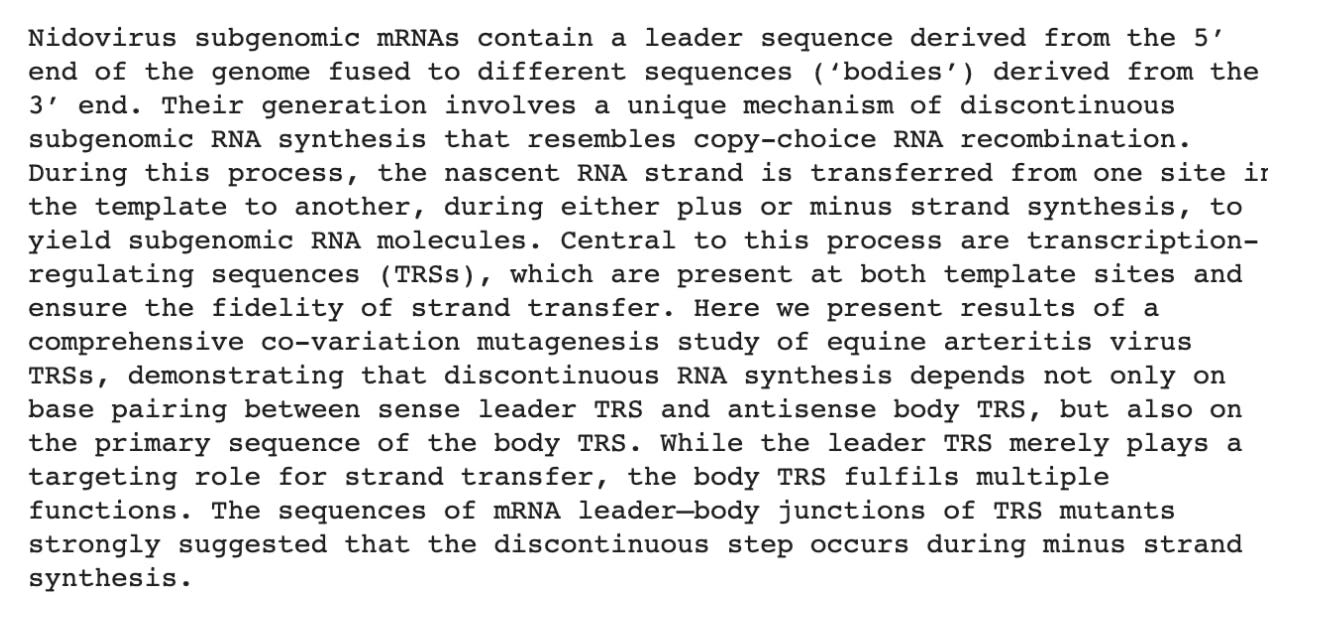
This finds the abstract located in the first row of the table (remember, in Python indexing starts at 0) You can then print your newly created string to verify you have the data you want. If you copy this example, your text should look like this:

Implementing Named- Entity Recognition
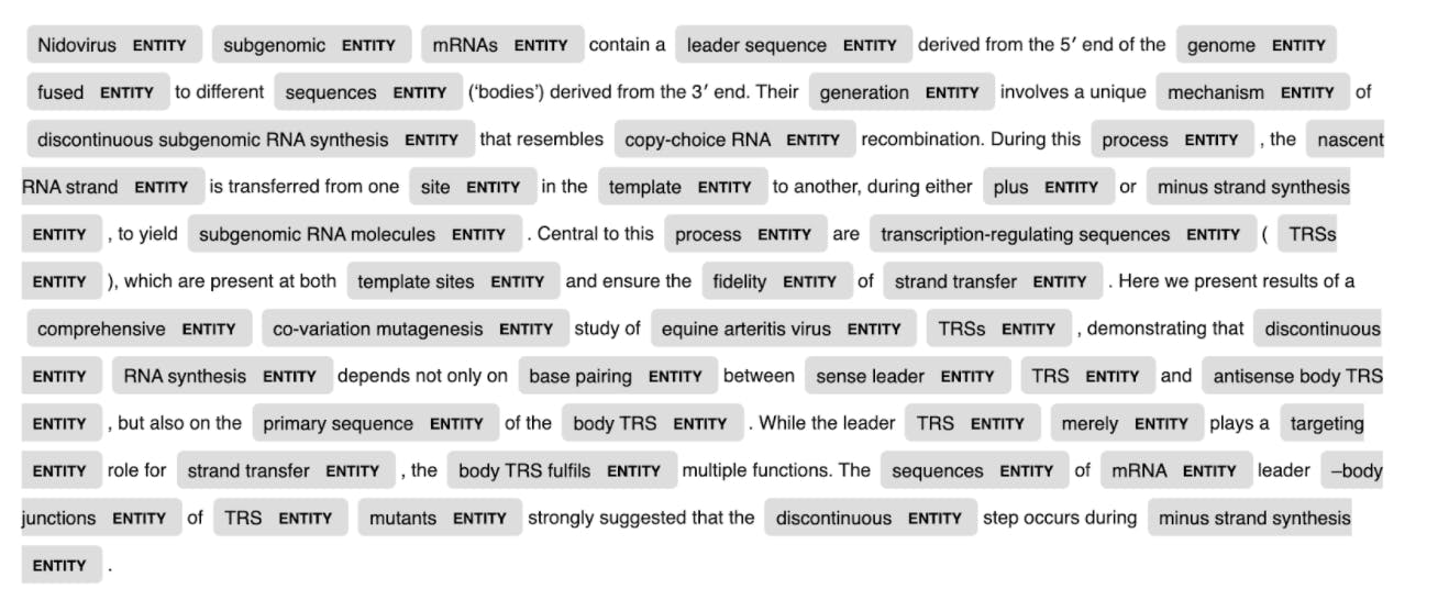
Now that you have your text, you can get into the fun part. Thanks to scispaCy, entity extraction is relatively easy. We will be using a Core model and a NER model to highlight the differences between the two.
Core model:
nlp = en_core_sci_sm.load()
doc = nlp(text)
displacy_image = displacy,render(doc, jupyter = True, style = ‘ent’)
Your output should look like this:

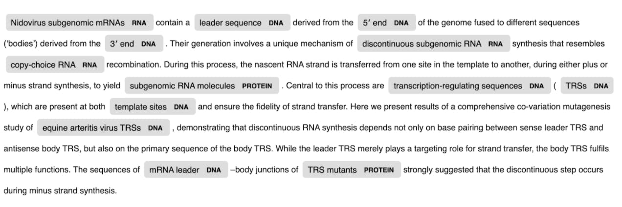
NER model:
nlp = en_ner_jnlpba_md.load()
doc = nlp(text)
displacy_image = displacy,render(doc, jupyter = True, style = ‘ent’)
This model is designed to identify entities of the type DNA, Cell Type, RNA, Protein, Cell Line
The output should look like this:

Expanding to Larger Data
Just like that, you have successfully used NER on a sample text! But, that was only one abstract of the over 60,000 in the CORD-19 metadata. What if we wanted to use NER on 100 abstracts? What about 1,000? What about all of them? Well, the process, though requiring a little more finesse, is essentially the same as before.
I highly recommend following along with the Google Colab project for these next steps to fully understand how we change the implementation to scan the entirety of the metadata.
So, the first step is the same as before. We need to read in our data.
meta_df = pd. read_csv(“/content/metadata.csv”)
Again use the specific path to the metadata file
Next, we load in our models. For this example, we are going to use all 4 NER models, so you’ll need to install and import them if you haven’t already. Just follow the instructions as described earlier.
nlp_cr = en_ner_craft_md.load()
nlp_bc = en_ner_bc5cdr_md.load()
nlp_bi = en_ner_bionlp13cg_md.load()
nlp_jn = en_ner_jnlpba_md.load()
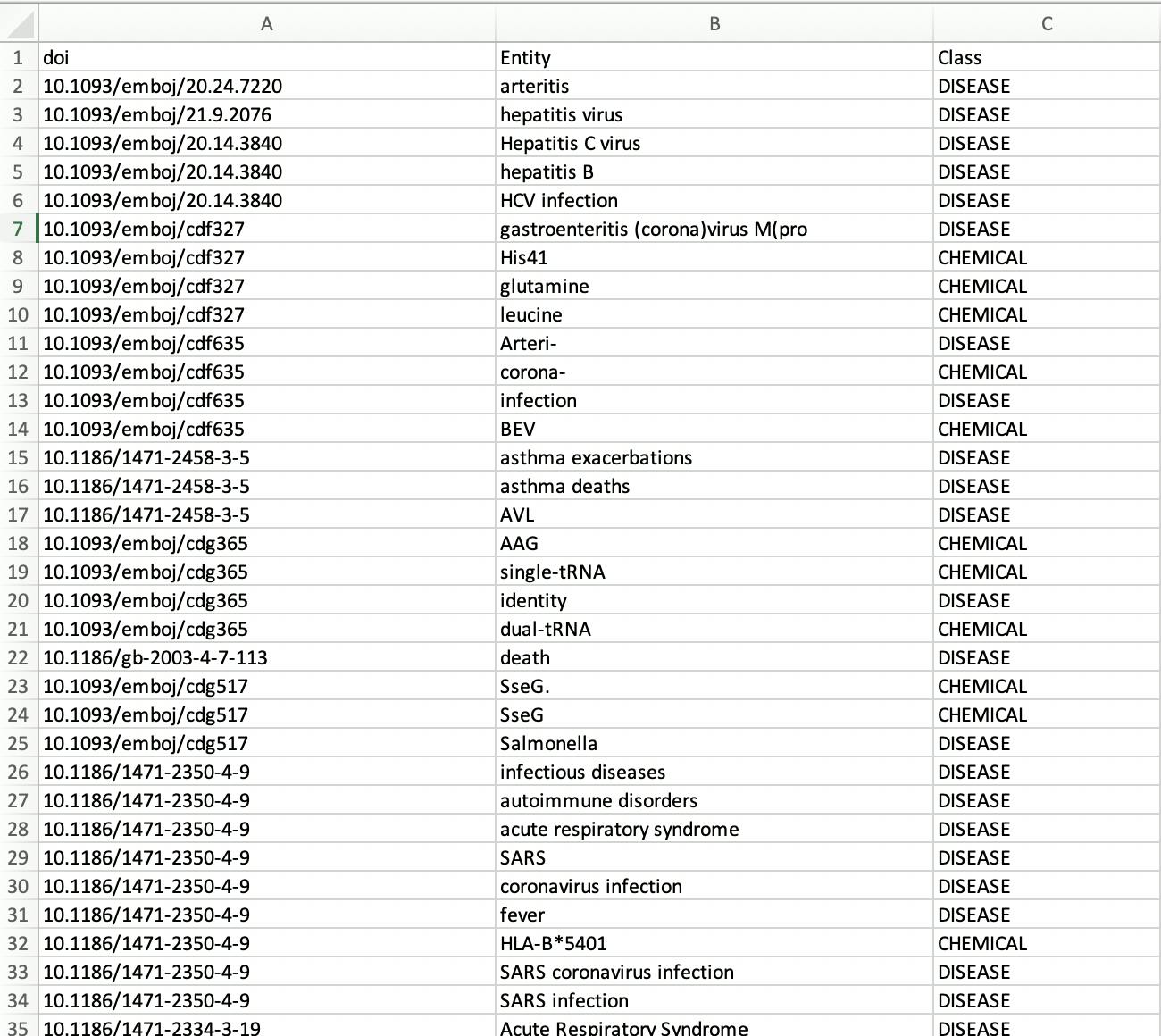
Now we want to create an empty table that will store the entity and value pairs. The table will have 3 columns: “doi”, “entity”, and “class”. The table will be normalized so that the doi for every entity/class pair will be in the “doi” column, even if that doi has already been listed. This is done so that there are no blank spaces in any of the columns, which helps if you want to use the data for other programs. To create the table, you need to create a dictionary with 3 lists inside.
table= {"doi":[], "Entity":[], "Class":[]}
This is where things get a little complicated. We’ll start by looping over the entire file. To do this, we use the pandas index function, which gives you the range of values (the number of rows. We then use the itterrows() function to iterate over the entire file. So, your loop should look something like this.
meta_df.index
for index, row in meta_df.iterrows():
For each iteration of the loop, we want to extract the relevant abstract and doi. We also want to ignore any empty abstracts. The empty cells are stored as NaNs in Python, which have the type float.
text = meta_df.loc[index, "abstract"]
doi = meta_df.loc[index, "doi"]
if type(text) == float:
       continue
Now that we have our text, we need to use one of our models loaded earlier to extract the entities. In my code on Google Colab, this step is divided into separate methods, but it can also be written without the use of helper methods. Do note, however, that it is best to run the models one at a time, especially in Colab where reading and writing files take quite a long time. The conglomerate code using one of the 4 NER models should look something like this:
doc = nlp_bc(text)
ent_bc = {}
for x in doc.ents:
       ent_bc[x.text] = x.label_

for key in ent_bc:
       table["doi"].append(doi)
       table["Entity"].append(key)
       table["Class"].append(ent_bc[key])
Remember that all of this code is inside the initial for loop
This code might look scary, but in reality, it’s quite similar to what we’ve already practiced. We pass our text through a model, but this time instead of displaying the result using displacy, we store it in a dictionary. We then loop through the dictionary and append the results, along with the corresponding doi of the article we are looking at, to our table. We continue to do this, looping over every row in the file. Once the table is filled, and our for loop is complete, the last step is to create an output CSV file. Thanks to pandas, this is quite easy.
trans_df = pd.DataFrame(table)
trans_df.to_csv ("Entity.csv", index=False)
You can choose any title for the output file, as long as it follows the format shown. Once your code is done running, the output file will show up in the “Files” section on Google Colab. You can then download the file and admire all of your hard work.

Conclusion
If you followed along with this post, Congratulations! You just made your first step in the world of scispaCy and NER for scientific documents; however, there’s so much more to explore. Within scispaCy alone, there are methods for abbreviation detection, dependency parsing, sentence detection, and much more. I hope you enjoyed learning a little about scispaCy and how it can be used for biomedical NLP, and I hope you all continue to play around, explore, and learn.
Resources:
